Click on the Time series icon, which will redirect you into the project creation screen. This will take the users into the screen where the project can be created. User can create a project as same as data analytics.
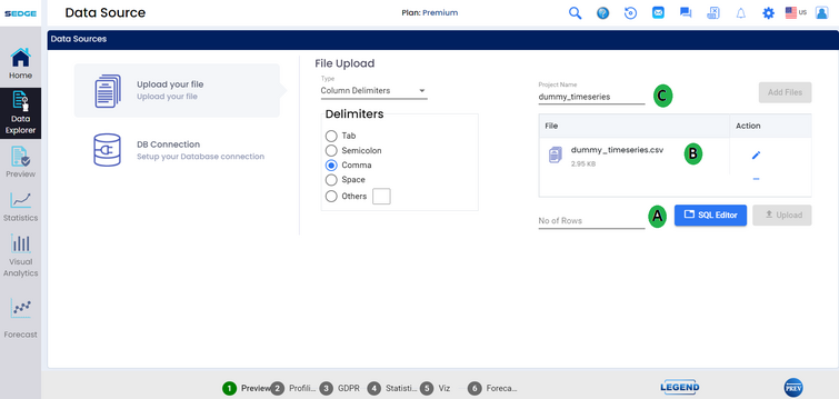
A - After adding your files, which might take a while, depending on the file size, click on the SQL Editor button, which will redirect you to the SQl query generator.
B - Users also have the option of zipping the CSV file, as large size CSV file can be uploaded.
C - Users can enter the name of the project (optional). If the users have not entered the name of the file then the system will take the name of the file and set a default project number.
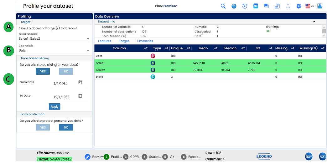
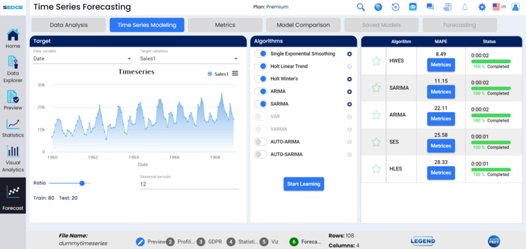
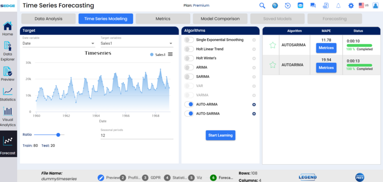
A - In this section , we can select one or more targets to run univariate or multivariate time series forecasting.
B - A date must be selected in order to forecast the future values. Since time series is pattern learning in time interval date. We can also see how data is distributed over time. It is highly important that the date should be at regular intervals.
C - Slicing - A functionality to perform a sequential sampling especially when we have some noise data for a certain period or the data size is more that what we needed.User can see the distribution of data pints over time and sample or slice accordingly.
If you wish to sample your data, after clicking “yes” you have to choose respective periods (By default it displays the start and end dates read from the dataset)
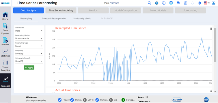
Resampling is used to resample the data, for example changing the intervals or frequency from a monthly basis to a yearly basis, down-sample method. There is also up-sample method functionality, allowing for a higher data frequency, such as from a monthly to a daily basis. Resampling types include linear, spline, polynomial, cubic, and quadratic algorithms.
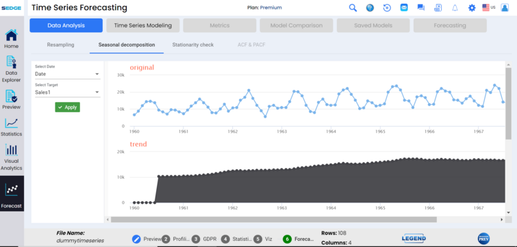
Seasonal decomposition functionality identifies the potential bias in the data, which allows the data analyst to easily identify trends over time, differentiating between seasonality and trends.
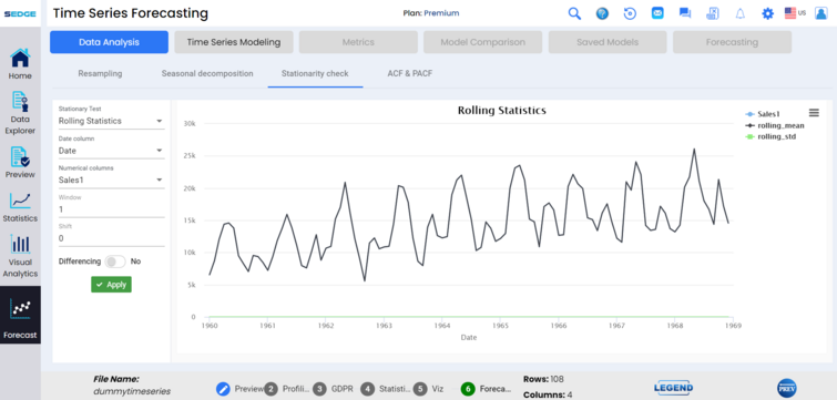
Stationarity checks allow data analysts to identify potential bias due to the presence of great data fluctuations caused by seasonality. This is done by utilizing rolling statistics on the time series, as well as ADF test statistics and Johansen test capabilities. Once the data becomes stationary, the model can easily grasp the pattern.
The Kwiatkowski-Phillips-Schmidt-Shin (KPSS) test figures out if a time series is stationary around a mean or linear trend, or is non-stationary due to a unit root. A stationary time series is one where statistical properties — like the mean and variance — are constant over time.
The null hypothesis for the test is that the data is stationary.
The alternate hypothesis for the test is that the data is not stationary.
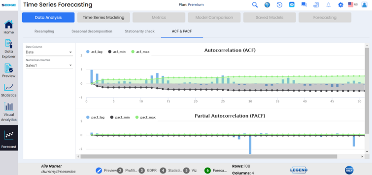
Data analysis functionality also includes ACF & PACF capabilities, showing autocorrelation (ACF) and partial autocorrelation (PACF) on the data.Auto correlation analysis measures the relationship of the data points between different points in time seeking for a patten or trend. ACF helps to find the degree of similarity between data points over time.
The simplest of the exponentially smoothing methods is naturally called simple exponential smoothing. Exponential smoothing is a forecasting method for univariate time series data. This method produces forecasts that are weighted averages of past observations where the weights of older observations exponentially decrease. Forms of exponential smoothing extend the analysis to model data with trends and seasonal components.
Note
The order of smoothing levels cannot be greater than 1.
Holt-Winters is a model of time series behavior. Forecasting always requires a model, and Holt-Winters is a way to model three aspects of the time series: a typical value (average), a slope (trend) over time, and a cyclical repeating pattern (seasonality).
The following descriptive acronym explains the meaning of each of the key components of the ARIMA model:
The “AR” in ARIMA stands for autoregression, indicating that the model uses the dependent relationship between current data and its past values. In other words, it shows that the data is regressed on its past values.
The “I” stands for integrated, which means that the data is stationary. Stationary data refers to time-series data that’s been made “stationary” by subtracting the observations from the previous values.
The “MA” stands for moving average model, indicating that the forecast or outcome of the model depends linearly on the past values. Also, it means that the errors in forecasting are linear functions of past errors.
The Autoregressive Integrated Moving Average (ARIMA) model uses time-series data and statistical analysis to interpret the data and make future predictions. The ARIMA model aims to explain data by using time series data on its past values and uses linear regression to make predictions. The ARIMA model is typically denoted with the parameters (p, d, q), which can be assigned different values to modify the model and apply it in different ways. Some of the limitations of the model are its dependency on data collection and the manual trial-and-error process required to determine parameter values that fit best. The ARIMA model is typically denoted with the parameters (p, d, q), which can be assigned different values to modify the model and apply it in different ways.
Each of the AR, I, and MA components are included in the model as a parameter. The parameters are assigned specific integer values that indicate the type of ARIMA model. A common notation for the ARIMA parameters is shown and explained below:
The parameter p is the number of autoregressive terms or the number of “lag observations”. It is also called the “lag order”, and it determines the outcome of the model by providing lagged data points.
The parameter d is known as the degree of difference. it indicates the number of times the lagged indicators have been subtracted to make the data stationary.
The parameter q is the number of forecast errors in the model and is also referred to as the size of the moving average window.
The parameters take the value of integers and must be defined for the model to work. They can also take a value of 0, implying that they will not be used in the model. In such a way, the ARIMA model can be turned into:
ARMA model (no stationary data, d = 0)
AR model (no moving averages or stationary data, just an autoregression on past values, d = 0, q = 0)
MA model (a moving average model with no autoregression or stationary data, p = 0, d = 0)
Therefore, ARIMA models may be defined as:
ARIMA(1, 0, 0) – known as the first-order autoregressive model
ARIMA(0, 1, 0) – known as the random walk model
ARIMA(1, 1, 0) – known as the differenced first-order autoregressive model, and so on.
Once the parameters (p, d, q) have been defined, the ARIMA model aims to estimate the coefficients α and θ, resulting from using previous data points to forecast values.
Seasonal Autoregressive Integrated Moving Average, SARIMA or Seasonal ARIMA, is an extension of ARIMA that explicitly supports univariate time series data with a seasonal component.
It adds three new hyperparameters to specify the autoregression (AR), differencing (I), and moving average (MA) for the seasonal component of the series, as well as an additional parameter for the period of the seasonality.
Four seasonal elements are not part of ARIMA that must be configured; they are:
The vector autoregressive (VAR) model is a workhouse multivariate time series model that relates current observations of a variable with past observations of itself and past observations of other variables in the system. The Vector Autoregression (VAR) model is a random process model that is used to capture the linear interdependence among the several series.
Auto_arima applies automated configuration tasks to the autoregressive integrated moving average (ARIMA) model. This model automatically discovers the optimal order for an ARIMA model with stepwise execution of hyperparameters and parallel fitting of models.
Auto-ARIMA combines auto-regression, differencing, and a moving average into a single model using the following steps
It checks whether differencing is required and identifies the optimal order for (d) if needed.
Using the optimal order for (d), it calculates the differences between consecutive observations to transform nonstationary data into stationary.
Using the selected information criterion and the optimal order for (d), it calculates various combinations of (p), (q), and (d) until it can identify the optimal order for (p) and (q). For example, a possible combination of orders is (2,1,3) for (p,d,q).
Using the optimal orders for (p) and (q), it calculates the forecast by applying autoregression and moving average on the differenced data.
The benefit of using Auto ARIMA over the ARIMA model is that we can skip the next steps & directly fit our model after the data preprocessing step. It uses the AIC (Akaike Information Criterion) & BIC(Bayesian Information Criterion) values generated by trying different combinations of p,q & d values to fit the model.
It is the Automatic estimate of the Seasonal ARIMA model. This returns the best seasonal ARIMA model using the start and end values.
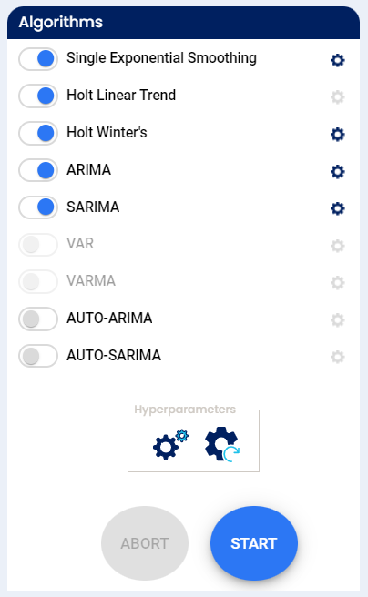
We can see the status of each algorithm, some of these are more complicated and will take more time. After all are at 100% of completion, the algorithms are sorted by their accuracy.
In our case, If user chooses 2 to 5 target variables, we can see 2 algorithms were used.
User selecting one target variable can enable other two models by clicking toggle button after clicking yes click yes , we can see 2 algorithms were used.
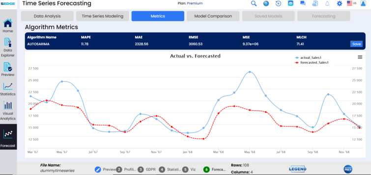
Actual vs. forecasted metrics allow data analysts to check the validity of their models to ensure learning is aligned with actuals, and that predictions will be accurate.
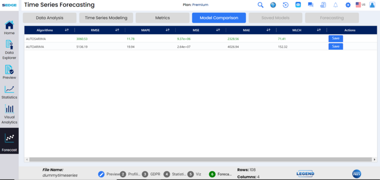
The SEDGE application now allows data analysts to review and compare models by MAPE (mean absolute percentage error), RMSE (root mean square error), MSE (mean squared error), MAE (mean absolute error), and MLCH. This allows the analyst to save and test models for greatest accuracy.